Interacting graphene

In the previous tutorial, we showed how to use MeanFi to solve a simple 1D Hubbard model with onsite interactions. In this tutorial, we will apply MeanFi to more complex system: graphene with onsite \(U\) and nearest-neighbour \(V\) interactions. The system is more complicated in every aspect: the lattice structure, dimension of the problem, complexity of the interactions. And yet, the workflow is the same as in the previous tutorial and remains simple and straightforward.

Building the system with kwant

Non-interacting part

As in the previous tutorial, we could construct a tight-binding dictionary of graphene by hand, but instead it is much easier to use kwant to build the system. For a more detailed explanation on kwant see the tutorial.

import kwant
import matplotlib.pyplot as plt
import meanfi
import numpy as np
from meanfi.kwant_helper import utils

s0 = np.identity(2)
sx = np.array([[0, 1], [1, 0]])
sy = np.array([[0, -1j], [1j, 0]])
sz = np.diag([1, -1])

# Create graphene lattice
graphene = kwant.lattice.general(
    [(1, 0), (1 / 2, np.sqrt(3) / 2)], [(0, 0), (0, 1 / np.sqrt(3))], norbs=2
)
a, b = graphene.sublattices

# Create bulk system
bulk_graphene = kwant.Builder(kwant.TranslationalSymmetry(*graphene.prim_vecs))
# Set onsite energy to zero
bulk_graphene[a.shape((lambda pos: True), (0, 0))] = 0 * s0
bulk_graphene[b.shape((lambda pos: True), (0, 0))] = 0 * s0
# Add hoppings between sublattices
bulk_graphene[graphene.neighbors(1)] = s0

Matplotlib is building the font cache; this may take a moment.

The bulk_graphene object is a kwant.Builder object that represents the non-interacting graphene system. To convert it to a tight-binding dictionary, we use the builder_to_tb function:

h_0 = utils.builder_to_tb(bulk_graphene)

Interacting part

We utilize kwant to build the interaction tight-binding dictionary as well. To define the interactions, we need to specify two functions:

• onsite_int(site): returns the onsite interaction matrix.

• nn_int(site1, site2): returns the interaction matrix between site1 and site2.

We feed these functions to the build_interacting_syst function, which constructs the kwant.Builder object encoding the interactions. All we need to do is to convert this object to a tight-binding dictionary using the builder_to_tb function.

def onsite_int(site, U):
    return U * sx

def nn_int(site1, site2, V):
    return V * np.ones((2, 2))

builder_int = utils.build_interacting_syst(
    builder=bulk_graphene,
    lattice=graphene,
    func_onsite=onsite_int,
    func_hop=nn_int,
    max_neighbor=1
)
params = dict(U=0.2, V=1.2)
h_int = utils.builder_to_tb(builder_int, params)

Because nn_int function returns the same interaction matrix for all site pairs, we set max_neighbor=1 to ensure that the interaction only extends to nearest-neighbours and is zero for longer distances.

Computing expectation values

As before, we construct Model object to represent the full system to be solved via the mean-field approximation. We then generate a random guess for the mean-field solution and solve the system:

filling = 2
model = meanfi.Model(h_0, h_int, filling=2)
int_keys = frozenset(h_int)
ndof = len(list(h_0.values())[0])
guess = meanfi.guess_tb(int_keys, ndof)
mf_sol = meanfi.solver(model, guess, nk=20)
h_full = meanfi.add_tb(h_0, mf_sol)

To investigate the effects of interaction on systems with more than one degree of freedom, it is more useful to consider the expectation values of various operators which serve as order parameters. For example, we can compute the charge density wave (CDW) order parameter which is defined as the difference in the charge density between the two sublattices.

To calculate operator expectation values, we first need to construct the density matrix via the density_matrix function. We then feed it into expectation_value function together with the operator we want to measure. In this case, we compute the CDW order parameter by measuring the expectation value of the \(\sigma_z\) operator acting on the graphene sublattice degree of freedom.

cdw_operator = {(0, 0): np.kron(sz, np.eye(2))}

rho, _ = meanfi.density_matrix(h_full, filling=filling, nk=40)
rho_0, _ = meanfi.density_matrix(h_0, filling=filling, nk=40)

cdw_order_parameter = meanfi.expectation_value(rho, cdw_operator)
cdw_order_parameter_0 = meanfi.expectation_value(rho_0, cdw_operator)

print(
    f"CDW order parameter for interacting system: {np.round(np.abs(cdw_order_parameter), 2)}"
)
print(
    f"CDW order parameter for non-interacting system: {np.round(np.abs(cdw_order_parameter_0), 2)}"
)

CDW order parameter for interacting system: 1.68
CDW order parameter for non-interacting system: 0.0

We see that the CDW order parameter is non-zero only for the interacting system, indicating the presence of a CDW phase.

Graphene phase diagram

In the remaining part of this tutorial, we will utilize all the tools we have developed so far to create a phase diagram for the graphene system.

To identify phase changes, it is convenient to track the gap of the system as a function of \(U\) and \(V\). To that end, we first create a function that calculates the gap of the system given the tight-binding dictionary and the Fermi energy.

def compute_gap(h, fermi_energy=0, nk=100):
    kham = meanfi.tb_to_kgrid(h, nk)
    vals = np.linalg.eigvalsh(kham)

    emax = np.max(vals[vals <= fermi_energy])
    emin = np.min(vals[vals > fermi_energy])
    return np.abs(emin - emax)

And proceed to compute the gap and the mean-field correction for a range of \(U\) and \(V\) values:

Us = np.linspace(0, 4, 10)
Vs = np.linspace(0, 1.5, 10)

gaps = []
mf_sols = []
for U in Us:
    for V in Vs:
        params = dict(U=U, V=V)
        h_int = utils.builder_to_tb(builder_int, params)

        model = meanfi.Model(h_0, h_int, filling=filling)
        guess = meanfi.guess_tb(int_keys, ndof)
        mf_sol = meanfi.solver(model, guess, nk=18)
        mf_sols.append(mf_sol)

        gap = compute_gap(meanfi.add_tb(h_0, mf_sol), fermi_energy=0, nk=100)
        gaps.append(gap)
gaps = np.asarray(gaps, dtype=float).reshape((len(Us), len(Vs)))
mf_sols = np.asarray(mf_sols).reshape((len(Us), len(Vs)))

plt.imshow(gaps.T, extent=(Us[0], Us[-1], Vs[0], Vs[-1]), origin="lower", aspect="auto")
plt.colorbar()
plt.xlabel("V")
plt.ylabel("U")
plt.title("Gap")
plt.show()

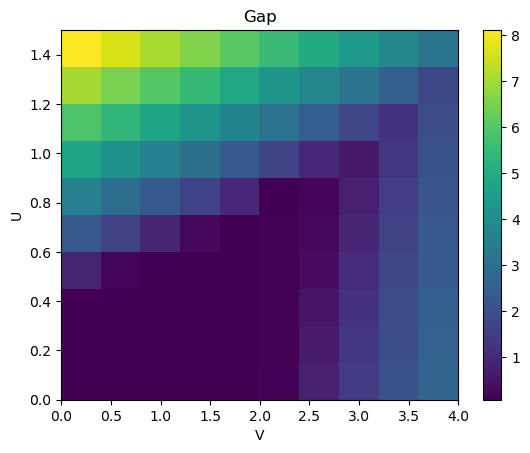
This phase diagram has gap openings at the same places as shown in the literature.

We can now use the stored results in mf_sols to fully map out the phase diagram with order parameters. On top of the charge density wave (CDW), we also expect a spin density wave (SDW) in a different region of the phase diagram. We construct the SDW order parameter with the same steps as before, but now we need to sum over the expectation values of the three Pauli matrices to account for the \(SU(2)\) spin-rotation symmetry.

s_list = [sx, sy, sz]
cdw_list = []
sdw_list = []
for mf_sol in mf_sols.flatten():
    rho, _ = meanfi.density_matrix(meanfi.add_tb(h_0, mf_sol), filling=filling, nk=40)

    # Compute CDW order parameter
    cdw_list.append(np.abs(meanfi.expectation_value(rho, cdw_operator)) ** 2)

    # Compute SDW order parameter
    sdw_value = 0
    for s_i in s_list:
        sdw_operator_i = {(0, 0): np.kron(sz, s_i)}
        sdw_value += np.abs(meanfi.expectation_value(rho, sdw_operator_i)) ** 2
    sdw_list.append(sdw_value)

cdw_list = np.asarray(cdw_list).reshape(mf_sols.shape)
sdw_list = np.asarray(sdw_list).reshape(mf_sols.shape)

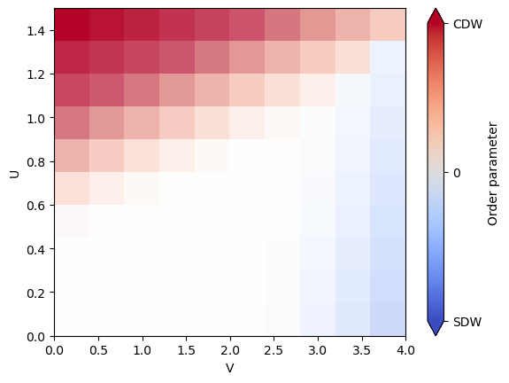
Finally, we can combine the gap, CDW and SDW order parameters into one plot. We naively do this by plotting the difference between CDW and SDW order parameters and indicate the gap with the transparency.

import matplotlib.ticker as mticker

normalized_gap = gaps / np.max(gaps)
plt.imshow(
    (cdw_list - sdw_list).T,
    extent=(Us[0], Us[-1], Vs[0], Vs[-1]),
    origin="lower",
    aspect="auto",
    cmap="coolwarm",
    alpha=normalized_gap.T,
    vmin=-2.6,
    vmax=2.6,
)
plt.colorbar(
    ticks=[-2.6, 0, 2.6],
    format=mticker.FixedFormatter(["SDW", "0", "CDW"]),
    label="Order parameter",
    extend="both",
)
plt.xlabel("V")
plt.ylabel("U")
plt.show()