Strained graphene superlattice

We showcase the interface between meanfi and Kwant with a strained graphene supercell. In this tutorial, we qualitatively reproduce the results from [1].

We first create the atomistic model in Kwant. The complete source code of this example can be found in strained_graphene_kwant.py. To reduce the computational cost, we perform the calculations with a \(16 \times 16\) supercell whereas in 1 the calculations were performed with a \(25 \times 25\) supercell. Thus, the agreement throughout the tutorial is only qualitative.

Show code cell source Hide code cell source

import kwant
import matplotlib.pyplot as plt
import meanfi
import numpy as np
from meanfi.kwant_helper import utils
from scripts.pauli import s0, sx, sy, sz
from scripts.strained_graphene_kwant import create_system, plot_bands

sigmas = [sx, sy, sz]

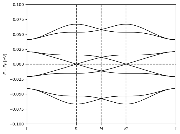
We verify the band structure of the Kwant model along a high-symmetry k-path.

h0_builder, lat, k_path = create_system(n=16)

Show code cell source Hide code cell source

fsyst = kwant.wraparound.wraparound(h0_builder).finalized()
params = {"xi": 7}


def hk(k):
    return fsyst.hamiltonian_submatrix(
        params={**params, **dict(k_x=k[0], k_y=k[1])}, sparse=False
    )


plot_bands(hk, k_path)

We now use the Kwant model to create the interacting Hamiltonian. Following [1], we consider only onsite interactions.

def func_hop(site1, site2):
    return 0 * np.ones((2, 2))


def func_onsite(site, U):
    return U * np.ones((2, 2))


int_builder = utils.build_interacting_syst(
    h0_builder,
    lat,
    func_onsite,
    func_hop,
    max_neighbor=0,
)

After we have created the interacting system we can use MeanFi again for getting the solution. We turn both the non-interacting and interacting systems into tight binding dictionaries using the kwant utils. Then we combine them into a mean-field model.

from meanfi.kwant_helper import utils as utils

h0, data = utils.builder_to_tb(h0_builder, params={"xi": 7}, return_data=True)

params_int = dict(U=0.8)
ndof = [*h0.values()][0].shape[0]
filling = ndof // 2
h_int = utils.builder_to_tb(int_builder, params_int)
mf_model = meanfi.Model(h0, h_int, filling=filling)

Now getting the solution by providing a guess and the mean-field model to the solver. To accelerate the convergence, we use an antiferromagnetic guess.

def func_hop(site1, site2):
    return 0 * np.ones((2, 2))


def func_onsite(site):
    if site.family == lat.sublattices[0]:
        return sz
    else:
        return -sz


guess_builder = utils.build_interacting_syst(
    h0_builder,
    lat,
    func_onsite,
    func_hop,
    max_neighbor=0,
)

guess = utils.builder_to_tb(guess_builder)

Due to the large supercell, lwe use a coarse k-point grid. Furthermore, to speed up the calculation we provide additional optimizer_kwargs.

mf_sol = meanfi.solver(
    mf_model,
    guess,
    nk=2,
    optimizer_kwargs={
        "M": 10,
        "f_tol": 1e-4,
        "maxiter": 100,
        "line_search": "armijo",
    },
)

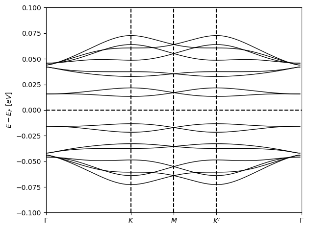
We now verify that the mean-field solution results in a gapped phase.

mf_ham = meanfi.add_tb(h0, mf_sol)
hk_mf = meanfi.tb_to_kfunc(mf_ham)
plot_bands(hk_mf, k_path)

Now we turn the mean-field corrections into a kwant.Builder such that we can visualize observables using Kwant’s functionalities. We provide the mean-field solution mf_sol as well as the sites and periods of the bulk system to the tb_to_builder function.

mf_sol_builder = utils.tb_to_builder(mf_sol, data["sites"], data["periods"])

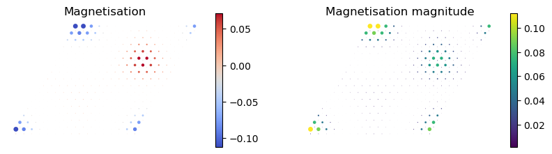
We now plot the magnetization of the system. First, we define the magnetization direction. We do extracting the exchange field at it site and finding the direction where all the spins are pointing to.

exchange_field = np.array([value[1] for value in list(mf_sol_builder.site_value_pairs())])

magnetization_direction = np.zeros(3)
for i, sigma in enumerate(sigmas):
    for site_field in exchange_field:
        magnetization_direction[i] += np.abs(np.trace(sigma @ site_field))

magnetization_direction /= np.linalg.norm(magnetization_direction)
reference_magnetization = np.transpose(sigmas, (1, 2, 0)) @ magnetization_direction

Now we plot the magnetization of the solution on the sites of the system. We do this by creating functions which calculate the magnetization and its magnitude with respect to the reference magnetization direction.

def magnetisation(site):
    matrix = mf_sol_builder.H[site][1]
    return np.trace(reference_magnetization @ matrix).real


def abs_magnetisation(site):
    matrix = mf_sol_builder.H[site][1]
    projected_magnetization = []
    for sigma in sigmas[1:]:
        projected_magnetization.append(np.trace(sigma @ matrix))
    return np.sqrt(np.sum(np.array(projected_magnetization) ** 2).real)


def systemPlotter(syst, onsite, ax, cmap):
    """
    Plots the system with the onsite potential given by the function onsite.
    """
    sites = [*syst.sites()]
    density = [onsite(site) for site in sites]

    def size(site):
        return 0.3 * np.abs(onsite(site)) / np.max(np.abs(density))

    kwant.plot(
        syst, site_color=onsite, ax=ax, cmap=cmap, site_size=size, show=False, unit=1
    )
    return np.min(density), np.max(density)

Show code cell source Hide code cell source

import matplotlib
from mpl_toolkits.axes_grid1 import make_axes_locatable

fig, axs = plt.subplots(1, 2, figsize=(10, 5))


titles = ["Magnetisation", "Magnetisation magnitude"]
cmaps = ["coolwarm", "viridis"]
onsites = [magnetisation, abs_magnetisation]
for i, ax in enumerate(axs):
    vmin, vmax = systemPlotter(mf_sol_builder, onsites[i], ax=ax, cmap=cmaps[i])
    ax.axis("off")
    ax.set_title(titles[i])
    ax.set_aspect("equal")
    fig.colorbar(ax.collections[0], ax=ax, shrink=0.5)
fig.show()

/home/docs/checkouts/readthedocs.org/user_builds/meanfi/conda/latest/lib/python3.11/site-packages/kwant/_plotter.py:77: RuntimeWarning: plotly is not available, if other engines are unavailable, only iterator-providing functions will work
  warnings.warn("plotly is not available, if other engines are unavailable,"